My first step to go into Deep

Another post starts with you beautiful people!
From this post I am going to share my learning from the data camp and various sources about the Deep Learning- a subfield of machine learning inspired by the structure and function of the brain (called artificial neural networks). Before jumping into the Python code, we must understand nuts and bolts of Deep Learning. That is what we are going to learn in this post.

When you hear the term Deep Learning, just think of a large deep neural network. This network is so much powerful is that Deep Learning gives amazing results for text, images, audio and video data. For every problem, deep learning models capture interactions and how they capture the interactions we need to understand following three components-

1. Input Layer:- situated in far left side in neural network and represents our predictive features.
2. Output Layer:- situated in far right side and represents the prediction from our model
3. Hidden Layer:- all layers that are not input or output layers, generally situated between the input and output layers. Each neuron or node in the hidden layer represents an aggregation of information from our input data and answers the model's ability to capture interactions. So more nodes we have means more interactions we capture. Don't worry, as a modeler you don't need to specify the interactions, deep learning will do it for yourself.

Following image shows an example of neural network model-

And following image example shows a  single artificial neuron that receives input from one or more sources being other neurons or data input-

The node or artificial neuron multiplies each of these inputs by a weight. Then it adds the multiplications and passes the sum to an activation function. Some neural networks do not use an activation function when their principle is different. One important point with respect to neural network model is that the data can be binary, integers or floating point values but if a symbolic or nominal variable is there in data, this must first be encoded with a set of binary variables.

Forward Propagation:- Now we will understand how a neural network models use data to make prediction? This is also called Forward Propagation. The Forward Propagation algorithm pass the input layer information through the network to make a prediction in the output layer. Here lines connect the inputs to the hidden layer. Each line has a weight indicating how strongly that input affect the hidden node. These weights are the parameters we train or change when we fit our neural network model to the data.

See an example of bank transaction in above image. A person has 2 children and 3 accounts in a bank where we have 1 weight from the top input into the top node of the hidden layer and 1 weight from the bottom input to the top node of the hidden layer. Now to make prediction to the top node of the hidden layer, we take the value of each node in the input layer multiplied by the weight that end that node and then sum of all those values. In our case we will get: (2 x 1) + (3 x 1) that is 5; similarly in the bottom we will get: (2 x -1) + (3 x 1) that is 1 as shown in below image-

Finally we apply the same logic to the next layer in our case it is output layer and we will get: (5 x 2) + (1 x -1) that is output of prediction 9-

So you have made prediction that the person may do 9 transaction in next year. The above multiply-add process is known as Forward Propagation for a single data point. The same logic we can achieve through Pandas numpy as shown below-

Quite amazing right! You have made the prediction using pen or pencil as well as using Pandas also. Since this is a single data point it was easy for us to calculate it with pen or pencil. In real world problems (mostly no-linear) there are so many layers exist so to get the maximum power of a neural network we apply activation function in the hidden layers. An activation function allows the model to capture the non-linear-ties. Non-linearties example in our case is how an account from children 2 to 3 may impact your banking transaction than from 3 children to 4 children.

An activation function is applied to value coming into a node which then transforms into a value stored in that node or the node output. In other words the activation function is the non linear transformation that we do over the input signal. This transformed output is then sent to the next layer of neurons as input. Always remember that a neural network without an activation function is essentially just a linear regression model and a linear transformation cannot do complex task such as image classification. That's why to capture non-linearties we need an activation function.

Let's understand following most used activation functions and their use-

1. Sigmoid Activation Function:- It is an activation function of form f(x) = 1 / 1 + exp(-x) . Its Range is between 0 and 1 having S  shaped curve. It is usually used in output layer of a binary classification, where result is either 0 or 1, as value for sigmoid function lies between 0 and 1 only so, result can be predicted easily to be 1 if value is greater than 0.5 and 0 otherwise. This is a smooth function and is continuously differential means, we can find the slope of the sigmoid curve at any two points. One issue with this function is that sigmoid function is not symmetric around the origin and the values received are all positive. So not all times would we desire the values going to the next neuron to be all of the same sign.

2. Hyperbolic Tangent or Tanh fActivation Function:- Tanh activation function addresses the issue of the sigmoid activation function mentioned above. It is a scaled version of the sigmoid function. The range of the tanh function is from (-1 to 1) having S shaped curve. The equation of this function is tanh(x) = 2/(1 + exp(-2x)) - 1 OR tanh(x) = 2 * sigmoid(2x) - 1. It is used in hidden layers of a neural network as it’s values lies between -1 to 1 hence the mean for the hidden layer comes out be 0 or very close to it, taht's why it helps in centering the data by bringing mean close to 0. This makes learning for the next layer much easier.

3. ReLU:- Rectified Linear Unit or ReLU activation function the most used activation function in the world right now. This function takes a single number as an input and returns zero of the input is negative otherwise the input itself if input is positive. This function ranges from 0 to infinity. ReLU is less computationally expensive than tanh and sigmoid because it involves simpler mathematical operations. At a time only a few neurons are activated making the network sparse making it efficient and easy for computation. One issue with this activation function is- since it turns negative value to zero; it can create dead neurons which never get activated and one limitation of this function is that it should only be used within Hidden layers of a Neural Network Model.

4. Softmax Activation Function:- The softmax function is ideally used when trying to handle multiple classes. The Softmax layer must have the same number of nodes as the output layer. This activation function takes any vector of numbers, exponentiation everything, then divides every element by the sum of the exponential. In Softmax, every component is between 0 and 1 since an exponential can’t be negative and a division over the sum can’t be over 1 so the sum of output always be equal to 1.

Now we will see how can we use an activation function in our banking transaction example code. See previous code again and check the line where we have calculated values of node 0 and node 1 and passing these values to calculate hidden layer values. Now instead we will pass the input nodes values to an activation function and then we pass it to hidden layers as below-

In this example tanh activation function is giving prediction of 1.2 transactions.

Let's see how can we use Relu activation function instead of tanh in the same code example. Remember this function takes a single number as an input, returning 0 if the input is negative, and the input if the input is positive-

Great! It was quite easy right. In our example there was only 1 hidden layer but it can be 3, 10 or further more deep as per your problem. One of the advantage of the deep networks is that it internally build representation of the patterns in the data and thus it partially replace the feature engineering step while building your model. In deep network subsequent layers build increasingly sophisticated representations of the raw data. It means the last layers capture the most complex interactions.

Loss function:- Once we increase the weights in our neural network model, it also gets harder to make accurate predictions and this generates error in our predicted model. To aggregate errors in predictions from various data points into a single number we need a function and that's where loss function comes in the picture. The log function measures our model's prediction performance. For example a common loss function in regression task is 'mean squared error (MSE)' loss function.

Gradient Descent:- A lower loss function value means a better model, Gradient Descent algorithm helps us to find the weights that gives the lowest value for  the loss function. With Gradient Descent, we repeatedly find a slope capturing how our loss function changes as the weight changes. Then we make a small change to the weight to get a lower point and we keep repeating this till we find our goal. In this step if slope is positive then going opposite the slope means moving to the lower numbers. Subtracting the slope from the current value achieve this. But too big step might lead to a wrong direction. To solve this we update each weight by subtracting learning rate * slope and this solution is known as learning rate. Learning rate ensures we take snall steps and lead to an optimal result.

Slope Calculation Steps:- To calculate the slope for a weight, we need to multiply following three things:

1. Slope of the loss function with respect to value at the node we feed into
2. The value of the node that feeds into our weight
3. Slope of the activation function with respect to value we feed into

Let's see the code to calculate slopes and update weights:-

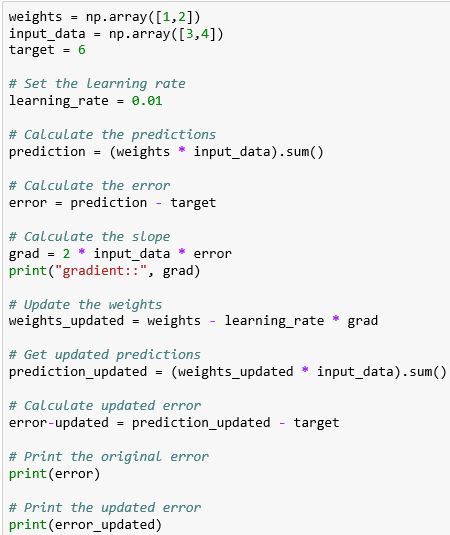
As you can see updating the weights decreases the error!

Backpropagation:- Backpropagation is a technique to calculate the slope we need to optimize more complex deep learning model. It takes the error from the output layer and propagates backwards through the hidden layers towards the input layers. In a nutshell with this technique we try to estimate the slope of the loss function with respect to each weight. So we always do forward propagation to make predictions and calculate errors before we do back propagation. In Back propagation process we go back one layer at a time. The three things we need to multiply to get the slope for weights are:

1. The value of the weights input nodes
2. Slope of the loss function with respect to node it feeds into
3. Slope of the activation function at the node it feeds into

In this process we also need to keep track of the slopes of the loss function with respect to node values. Slope of the node values are the sum of the slopes for all weights that come out of them. For understanding this multiplication, see the below example and assume that we have Relu as activation function, actual target value is 4 and error is 3-

The relevant slope for the output node will be 2 time the  error means (2 * 3 = 6) and slope of the activation function is 1 since output node is positive. So the slope for top weight is (1 * 6 = 6) and slope for bottom weight is (3 * 6 = 18).

Since deep network models seeks more computational power, computational efficiency is required in Backpropagation technique. That's why we calculate slopes on only a subset of the data known as batch then we use different batch of data to calculate the next update. Once we have used all the batches of the data we start over again at beginning. Each time through the data is called an epoch. Here we are calculating the slopes on one batch at a time. This technique is also known as Stochastic Gradient Descent.

As we have read neural network models require more computational power, training such models in a CPU is not recommended. Instead we should use GPU (graphics processing units). Don't worry you don''t need to buy a new laptop or pay for the GPU. Many cloud platform provide the GPU setup with some storage as free. In our case I am going to tell you about Google's Colab- a free Jupyter notebook environment that requires no setup and runs entirely in the cloud. Colab uses your Google drive so you can easily upload your datasets, jupyter notebook and files form github url. 

I am assuming you have a gmail account and you have logged in with this account. Next, you just need to go Google Colab Link and it will show a pop up with options like Examples, Recent, Google Drive, Github and Upload like below-

You can close this pop up and go to the File to create a new python 3 notebook; it will take few seconds and your new Python 3 notebook is ready. It is quite similar to your jupyter notebook and supports all the commands you have used there. So just go and rename your colab notebook. Now to use GPU in this notebook you need to go to the Edit ---> Notebook settings or Runtime>Change runtime type and select GPU as Hardware accelerator-

That's it now you can achieve the power of GPU while training your neural network model. That's it for today. In next post we will see how to use keras interface to create and optimize a deep learning model to the TensorFlow (a deep learning library). Till then Go chase your dreams, have an awesome day, make every second count and see you later in my next post.