
Another post starts with you beautiful people!
I am very happy that you have enjoyed my previous post about Decision Tree and Random Forest
and a lot of aspiring data scientists like You have asked me questions like tell a case study and how to apply our knowledge to a competition like in Kaggle?
So here I am! In this exercise we will work on a great dataset- Titanic disaster which we have studied in one of my earlier post. I suggest you to do a quick revision of that post here- Let me revise Titanic disaster and submit our prediction to Kaggle.
When the Titanic sank, 1502 of the 2224 passengers and crew were killed.
One of the main reasons for this high level of casualties was the lack of lifeboats on this self-proclaimed "unsinkable" ship.
In this course, we will learn how to apply machine learning techniques to predict a passenger's chance of surviving.
Let's start with loading in the training and testing set into our Python environment.
We will use the training set to build our model, and the test set to validate it.

Well done! Now that our data is loaded in, let's see if we can understand it.
Understanding our data-
Before starting with the actual analysis, it's important to understand the structure of our data.
Both test and train are DataFrame objects, the way pandas represent datasets.
We can easily explore a DataFrame using the .describe() method. .describe() summarizes the columns/features of the DataFrame, including the count of observations, mean, max and so on. Another useful trick is to look at the dimensions of the DataFrame. This is done by requesting the .shape attribute of our DataFrame object. (ex. your_data.shape)
If you examine the training set has 891 observations and 12 variables, count for Age is 714.


How many people in our training set survived the disaster with the Titanic?
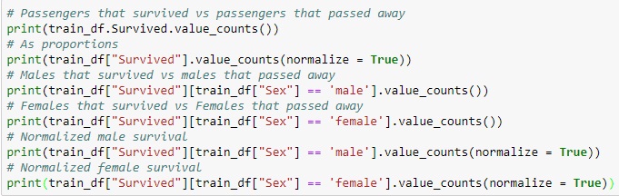
To see this, we can use the value_counts() method in combination with standard bracket notation to select a single column of a DataFrame:

If you run these commands in the console, you'll see that 549 individuals died (62%) and 342 survived (38%).
To dive in a little deeper we can perform similar counts and percentage calculations on subsets of the Survived column.

Does age play a role?
Another variable that could influence survival is age; since it's probable that children were saved first.
We can test this by creating a new column with a categorical variable Child.
Child will take the value 1 in cases where age is less than 18, and a value of 0 in cases where age is greater than or equal to 18.
To add this new variable we need to do two things (i) create a new column, and (ii) provide the values for each observation (i.e., row) based on the age of the passenger.
Adding a new column with Pandas in Python is easy and can be done via the following syntax:
your_data["new_var"] = 0
This code would create a new column in the train DataFrame titled new_var with 0 for each observation.


First Prediction-
Above we discovered that in our training set, females had over a 50% chance of surviving and males had less than a 50% chance of surviving.
Hence, we could use this information for our first prediction: all females in the test set survive and all males in the test set die.We use our test set for validating our predictions.
We might have seen that contrary to the training set, the test set has no Survived column.
We add such a column using our predicted values.

Key Note:-Before predicting you must clean your data otherwise you will get errors like TypeError,ValueError,NotFittedError. For this exercise I am not covering all cleaning code snippet.
Cleaning and Formatting our Data-
Before we can begin constructing our trees we need to get our hands dirty and clean the data
so that we can use all the features available.
In the previous, we saw that the Age variable had some missing value.
Missingness is a whole subject with and in itself, but we will use a simple imputation technique
where we substitute each missing value with the median of the all present values.
Another problem is that the Sex and Embarked variables are categorical but in a non-numeric format.
Thus, we will need to assign each class a unique integer so that Python can handle the information.
Embarked also has some missing values which we should impute with the most common class of embarkation, which is "S".

Great! Now that the data is cleaned up a bit we are ready to begin building our first decision tree-
Conceptually, the decision tree algorithm starts with all the data at the root node and scans all the variables for the best one to split on.
Once a variable is chosen, we do the split and go down one level (or one node) and repeat.
The final nodes at the bottom of the decision tree are known as terminal nodes, and the majority vote of the observations in that node determine how to predict for new observations that end up in that terminal node.
One way to quickly see the result of our decision tree is to see the importance of the features that are included.
This is done by requesting the .feature_importances_ attribute of our tree object.
Another quick metric is the mean accuracy that we can compute using the .score() function with features_one and target as arguments.

Well done! Time to investigate our decision tree a bit more.
Interpreting our decision tree-
The feature_importances_ attribute make it simple to interpret the significance of the predictors we include.
Based on our decision tree, what variable plays the most important role in determining whether or not a passenger survived?
Yes it is Passenger Fare.
Time to make a prediction and submit it to Kaggle!
Predict and submit to Kaggle-
To send a submission to Kaggle we need to predict the survival rates for the observations in the test set.
In the last exercise, we created simple predictions based on a single subset.
Luckily, with our decision tree, we can make use of some simple functions to "generate" our answer without having to manually perform subsetting.
First, we make use of the .predict() method.
We provide it the model (my_tree_one), the values of features from the dataset for which predictions need to be made (test).
To extract the features we will need to create a numpy array in the same way as we did when training the model.
However, we need to take care of a small but important problem first. There is a missing value in the Fare feature that needs to be imputed.
Next, you need to make sure our output is in line with the submission requirements of Kaggle:
a csv file with exactly 418 entries and two columns: PassengerId and Survived.
Then use the code provided to make a new data frame using DataFrame(), and create a csv file using to_csv() method from Pandas.

Great! You just created your first decision tree. Download your csv file, and submit the created csv to Kaggle to see the result of your effort.
Overfitting and how to control it-
When we created our first decision tree the default arguments for max_depth and min_samples_split were set to None.
This means that no limit on the depth of our tree was set. That's a good thing right? Not so fast. We are likely overfitting.
This means that while our model describes the training data extremely well, it doesn't generalize to new data, which is frankly the point of prediction. Just look at the Kaggle submission results for the simple model based on Gender and the complex decision tree. Which one does better?
Maybe we can improve the overfit model by making a less complex model? In DecisionTreeRegressor, the depth of our model is defined by two parameters:
- the max_depth parameter determines when the splitting up of the decision tree stops.
- the min_samples_split parameter monitors the amount of observations in a bucket.
If a certain threshold is not reached (e.g minimum 10 passengers) no further splitting can be done.
By limiting the complexity of our decision tree we will increase its generality and thus its usefulness for prediction!

Great! We just created our second and possibly improved decision tree.
Download your csv file .Submit your updated solution to Kaggle to see how despite a lower .score you predict better.
Feature-engineering for our Titanic data set-
Data Science is an art that benefits from a human element. Enter feature engineering: creatively engineering our own features by combining the different existing variables.
While feature engineering is a discipline in itself, too broad to be covered here in detail,
we will have a look at a simple example by creating our own new predictive attribute: family_size.
A valid assumption is that larger families need more time to get together on a sinking ship, and hence have lower probability of surviving.
Family size is determined by the variables SibSp and Parch, which indicate the number of family members a certain passenger is traveling with.
So when doing feature engineering, we add a new variable family_size, which is the sum of SibSp and Parch plus one (the observation itself), to the test and train set.

Great! Notice that this time the newly created variable is included in the model.
Download your csv file, and submit the created csv to Kaggle to see the result of the updated model.
Random Forest analysis-

Interpreting and Comparing-
Remember how we looked at .feature_importances_ attribute for the decision trees?
Well, we can request the same attribute from our random forest as well and interpret the relevance of the included variables.
We might also want to compare the models in some quick and easy way.
For this, we can use the .score() method. The .score() method takes the features data and the target vector and computes mean accuracy of your model.
We can apply this method to both the forest and individual trees.
Remember, this measure should be high but not extreme because that would be a sign of overfitting.

Based on your finding in the above exercise determine which feature was of most importance, and for which model and submit your random forest model to Kaggle!
Comments
Post a Comment