Another post starts with you beautiful people!
Today we will learn about an important topic related to statistics.
Statistical inference is the process of deducing properties of an underlying distribution by analysis of data. Inferential statistical analysis infers properties about a population: this includes testing hypotheses and deriving estimates.
Statistics are helpful in analyzing most collections of data. Hypothesis testing can justify conclusions even when no scientific theory exists.
You can find more about this here- tell me more about Statistical_hypothesis_testing
Here our case study will be Average Experience of Data Science Specialization(DSS) batch taught in a leading University with Statistical Inference.
We will aim to study how accurately can we characterize the actual average participant experience (population mean) from the samples of data (sample mean). We can quantify the certainty of outcome through the confidence intervals.

Let's plot the distribution of experience-

Result:-

Estimating DSS Experience from samples:-

We are now drawing samples for 1000 times (NUM_TRIALS) and compute the mean each time. The distribution is plotted to identify range of values it can take. The original data has experience raging between 0 years and 20 years and spread across it.
 Result:-

The above plot is histogram of mean of samples for any given n.
As you vary n from 1 to 128 you will see the following summary for the Sampling Distribution of Mean chart-
n = 1, Mean = 10.301, Std Dev = 5.689, 5% Pct = 1.000, 95% Pct = 19.000
n = 2, Mean = 10.431, Std Dev = 3.984, 5% Pct = 4.000, 95% Pct = 17.000
n = 4, Mean = 10.388, Std Dev = 2.878, 5% Pct = 5.500, 95% Pct = 15.000
n = 8, Mean = 10.407, Std Dev = 2.031, 5% Pct = 7.000, 95% Pct = 13.875
n = 10, Mean = 10.455, Std Dev = 1.794, 5% Pct = 7.600, 95% Pct = 13.405
n = 16, Mean = 10.467, Std Dev = 1.372, 5% Pct = 8.188, 95% Pct = 12.688
n = 32, Mean = 10.470, Std Dev = 0.984, 5% Pct = 8.844, 95% Pct = 12.125
n = 64, Mean = 10.446, Std Dev = 0.693, 5% Pct = 9.297, 95% Pct = 11.609
n = 128, Mean = 10.451, Std Dev = 0.502, 5% Pct = 9.625, 95% Pct = 11.258
One important point is to note the trend in values of Std Dev in the above table as n increases.
As n increases the Std Dev of Sampling distribution of Mean reduces from 5.689 (n = 1) to 0.502 (n = 128).
As n increases the Sampling distribution of Mean looks more normal.
It is observed that when n >= 30 irrespective of the original distribution the Sampling distribution of Mean becomes normal distribution.
Definition of Central Limit Theorem:-
In probability theory, the central limit theorem (CLT) establishes that, for the most commonly studied scenarios, when independent random variables are added, their sum tends toward a normal distribution (commonly known as a bell curve) even if the original variables themselves are not normally distributed [Ref: Wikipedia]
The key point to note is that irrespective of the original distribution then sum (and hence average as well) of large samples tend towards normal distribution. This gives power to estimate the confidence intervals.
Normal distribution has following characteristics:_


Function to check if the true mean lies within 90% Confidence Interval:-

Getting the average experience estimate from sample and Confidence Intervals:-
Now given the sample size n we can estimate the sample mean and confidence interval. The confidence interval is estimated assuming normal distribution which really holds good when n >= 30.
When n is increased the confidence interval becomes smaller which implies that results are obtained with higher certainty.
Execute the code below multiple times and check how often the population mean of 10.435 will lie within 90% confidence interval. It should be on average 9 out of 10 times i.e 90%-

Hypothesis Testing(HT):-
Let us define the Hypotheses as follows:




Today we will learn about an important topic related to statistics.
Statistical inference is the process of deducing properties of an underlying distribution by analysis of data. Inferential statistical analysis infers properties about a population: this includes testing hypotheses and deriving estimates.
Statistics are helpful in analyzing most collections of data. Hypothesis testing can justify conclusions even when no scientific theory exists.
You can find more about this here- tell me more about Statistical_hypothesis_testing
Here our case study will be Average Experience of Data Science Specialization(DSS) batch taught in a leading University with Statistical Inference.
We will aim to study how accurately can we characterize the actual average participant experience (population mean) from the samples of data (sample mean). We can quantify the certainty of outcome through the confidence intervals.

Let's plot the distribution of experience-

Result:-

Estimating DSS Experience from samples:-

We are now drawing samples for 1000 times (NUM_TRIALS) and compute the mean each time. The distribution is plotted to identify range of values it can take. The original data has experience raging between 0 years and 20 years and spread across it.


The above plot is histogram of mean of samples for any given n.
As you vary n from 1 to 128 you will see the following summary for the Sampling Distribution of Mean chart-
n = 1, Mean = 10.301, Std Dev = 5.689, 5% Pct = 1.000, 95% Pct = 19.000
n = 2, Mean = 10.431, Std Dev = 3.984, 5% Pct = 4.000, 95% Pct = 17.000
n = 4, Mean = 10.388, Std Dev = 2.878, 5% Pct = 5.500, 95% Pct = 15.000
n = 8, Mean = 10.407, Std Dev = 2.031, 5% Pct = 7.000, 95% Pct = 13.875
n = 10, Mean = 10.455, Std Dev = 1.794, 5% Pct = 7.600, 95% Pct = 13.405
n = 16, Mean = 10.467, Std Dev = 1.372, 5% Pct = 8.188, 95% Pct = 12.688
n = 32, Mean = 10.470, Std Dev = 0.984, 5% Pct = 8.844, 95% Pct = 12.125
n = 64, Mean = 10.446, Std Dev = 0.693, 5% Pct = 9.297, 95% Pct = 11.609
n = 128, Mean = 10.451, Std Dev = 0.502, 5% Pct = 9.625, 95% Pct = 11.258
One important point is to note the trend in values of Std Dev in the above table as n increases.
As n increases the Std Dev of Sampling distribution of Mean reduces from 5.689 (n = 1) to 0.502 (n = 128).
As n increases the Sampling distribution of Mean looks more normal.
It is observed that when n >= 30 irrespective of the original distribution the Sampling distribution of Mean becomes normal distribution.
Definition of Central Limit Theorem:-
In probability theory, the central limit theorem (CLT) establishes that, for the most commonly studied scenarios, when independent random variables are added, their sum tends toward a normal distribution (commonly known as a bell curve) even if the original variables themselves are not normally distributed [Ref: Wikipedia]
The key point to note is that irrespective of the original distribution then sum (and hence average as well) of large samples tend towards normal distribution. This gives power to estimate the confidence intervals.
Normal distribution has following characteristics:_


Function to check if the true mean lies within 90% Confidence Interval:-

Getting the average experience estimate from sample and Confidence Intervals:-
Now given the sample size n we can estimate the sample mean and confidence interval. The confidence interval is estimated assuming normal distribution which really holds good when n >= 30.
When n is increased the confidence interval becomes smaller which implies that results are obtained with higher certainty.
Execute the code below multiple times and check how often the population mean of 10.435 will lie within 90% confidence interval. It should be on average 9 out of 10 times i.e 90%-

Hypothesis Testing(HT):-
Let us define the Hypotheses as follows:
- H0 : Average Experience of Current Batch & Previous batch are same
- H1 : Average Experience of Current Batch & Previous batch are different
Repeat the same steps for previous batch-


Result:-

Below code describes to do hypothesis testing based on the intuition from Sampling distribution of mean. There will be differences with exact math based on various conditions and assumptions made.

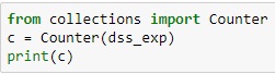
Show the frequency distribution of experience:-
Code for dumping the experiment results to a csv file:-

Demonstrate how the standard deviation of sample mean reduce and the distribution goes closer to normal distribution:-

Stats functions for Hypothesis Testing taken from here- hypothesis-testing-comparing-two-groups

ReplyDeleteAfter reading this blog i very strong in this topics and this blog really helpful to all.Data Science online Course Bangalore